CS91R Lab 08: GloVe vectors
Due Wednesday, April 23, before midnight
Goals
The goals for this lab assignment are:
-
Understand how cosine similarity is implemented
-
Get more experience working with pre-trained GloVe word vectors
-
Experiment with word2vec word vectors
-
Learn to use two dimensionality reduction techniques (PCA and t-SNE) to visualize word vectors
-
Learn to use geometric properties of vectors to make semantic predictions
Cloning your repository
Log into the CS91R-S25 github
organization for our class and find your git repository for Lab 08,
which will be of the format lab08-user1-user2, where user1 and user2
are you and your partner’s usernames.
You can clone your repository using the following steps while connected to the CS lab machines:
# cd into your cs91r/labs sub-directory and clone your lab08 repo
$ cd ~/cs91r/labs
$ git clone git@github.swarthmore.edu:CS91R-S25/lab08-user1-user2.git

# change directory to list its contents
$ cd ~/cs91r/labs/lab08-user1-user2

# ls should list the following contents
$ ls
README.md cosine.py visualize.py predict.py
Answers to written questions should be included in the README.md file included in your repository.
Background
In this lab, we will use two kinds of embeddings. The first set of embeddings we’ll use are GloVe vectors, which we’ve already seen in class. The other set is word2vec, use a similar dimensionality reduction technique to GloVe, but is trained differently.
Datasets
Both sets of data are already downloaded for you. These files are quite large. Do not copy these to your directory or check them into your repository.
The GloVe vectors are located in /data/cs91r-s25/glove. As downloaded from
the authors of the paper, these embeddings are in a text file. But, like we did
in clab, we have also created pickle files for you with the embeddings
stored in a pandas DataFrame. There are three pickle files we will use:
-
glove.6B.50d.pkl: 50-dimensional GloVe vectors trained on 6 billion tokens with 400K uncased (lowercased) types -
glove.42B.300d.pkl: 300-dimensional GloVe vectors trained on 42 billion tokens with 1.9M uncased (lowercased) types -
glove.840B.300d.pkl: 300-dimensional GloVe vectors trained on 840 billion tokens with 2.2M cased (mixed upper/lower case) types
The word2vec vectors are located in /data/cs91r-s25/word2vec. There is one
pickle file we will use:
-
GoogleNews-vectors-negative300.pkl: 300-dimensional word2vec vectors trained on 100 billion tokens with 3 million case (mixed upper/lower) types. Most of the types (approx 2 million) are multiword phrases joined using underscores. For example, "New_York" and "french_toast" are types in the word2vec embeddings. The remaining 1 million types are single words.
Cosine similarity
In the first part of the lab, you will write a program called cosine.py.
Before we begin coding, we will review how cosine similarity works
and see how to implement it ourselves.
In the last lab and in the clabs that used GloVe vectors, we used the
cosine_similarity function to compute the similarity between a query
(a single row of the matrix) and all of the other rows in the matrix:
from sklearn.metrics.pairwise import cosine_similarity # we won't use this in this lab
similarities = cosine_similarity(query, matrix).flatten()
In this lab, we’ll be using two functions from numpy to compute the
cosine similarity with the goal of giving you a better understanding of how
the cosine_similarity function works.
To find the cosine similarity between a query, \(u\), and a single row of the matrix, \(v\), you first compute the dot product of two vectors and then you divide by the length of the two vectors:
If you plan on repeating these calculations repeatedly, it is good to normalize each vector ahead of time. Normalizing a vector means setting the length of the vector to 1. To do this, you compute the length of the vector and then divide every value in the vector by the length of the vector. The length of a vector is defined as the square root of the sum of the squares of the values in the vector:
where \(v_i\) is the \(i\)th element of the vector \(v\), and \(n\) is the number of elements in the vector. In our case, the number of elements in the vector is the same as the number of columns in our matrix.
If the two vectors, \(u\) and \(v\), are already normalized, there is no need to divide by the lengths of the vectors when computing the cosine similarity since both lengths are 1. This simplifies the computation of the cosine similarity:
Normalizing the embeddings
At the top of your program, be sure you have the following line:
import numpy as npTo get the length of a vector, you can use the np.linalg.norm function.
For example:
row = embeddings.loc['banana']
length = np.linalg.norm(row)
You could put this in a loop and accumulate all of the lengths for every row,
but numpy can more efficiently calculate the lengths of every row in a matrix
if you provide the matrix as the second argument. You also need to provide
two optional arguments explained in the comment below:
#        axis=1: indicates you want to compute the length of each row (vs each column)
# keepdims=True: indicates you want the return type to be a matrix with the same
#                number of rows as the embeddings with one column storing the lengths
lengths = np.linalg.norm(embeddings, axis=1, keepdims=True)
Once you have all of the lengths, you can normalize all of the rows in the matrix by dividing the embeddings by the lengths:
normalized_embeddings = embeddings / lengthsWrite a function that takes your embeddings as a parameter and returns
the normalized_embeddings.
Implementing cosine similarity
Similar to the case with normalization, numpy provides code that will
compute the dot product between two vectors:
vec1 = normalized_embeddings.loc['banana']
vec2 = normalized_embeddings.loc['pineapple']
dot_product = vec1 @ vec2
And, just like with normalizing vectors, you could find the closest
match to "banana" by looping through all of the rows and acuumulating the
answer, but numpy can compute it more efficiently if you provide
the entire matrix at once:
similarities = vec1 @ normalized_embeddings.T # .T transposes the matrixWrite a function that takes a single normalized vector and your normalized embeddings as parameters and returns the cosine similarity. (This function will be very short!)
Verifying your solutions
If you are using the glove.6B.50d.pkl embeddings, you should be able
to duplicate these results, assuming you’ve named your functions the same
as I did and you’ve already loaded your embeddings into embeddings:
>>> normalized_embeddings = normalize(embeddings)
>>> sims = cosine(normalized_embeddings.loc['banana'], normalized_embeddings)
>>> print(sims.drop('banana').sort_values(ascending=False).head(10))
bananas      0.815203
coconut      0.787251
pineapple    0.757981
mango        0.755640
beet         0.721265
fruit        0.718141
sugar        0.718020
growers      0.716575
peanut       0.701811
cranberry    0.695799
Name: banana, dtype: float32
Building a command-line interface
When you run your cosine.py program from the command line, it should have the
following interface:
usage: cosine.py [-h] [-w WORD] [-f FILE] [-n NUM] pickle

Find the n closest words to a given word (if specified) or to all of the words
in a text file (if specified). If neither is specified, compute nothing.

positional arguments:
  pickle                path to glove vectors pickle

options:
  -h, --help            show this help message and exit
  -w WORD, --word WORD  a single word
  -f FILE, --file FILE  a text file with one-word-per-line
  -n NUM, --num NUM     find the top n most similar words
Be sure that your results do not include the target word. That is,
if you are searching for banana, as shown below, do not include the
word banana in your results.
If you want to find the 10 closest words to the word banana using the
glove.6B.50d.pkl vectors, you would write:
python3 cosine.py /data/cs91r-s25/glove/glove.6B.50d.pkl --word banana -n 10If you had a text file that had words (one per line) that you wanted to find the 5 closest for each of them, like the file shown below…
red
magenta
flower
plant
two
thousand
one
jupiter
mercury
oberlin
…then you could run this command to get the top 5 words for each of the words in your file (one after another):
python3 cosine.py /data/cs91r-s25/glove/glove.6B.50d.pkl --file words.txt -n 5Questions
-
For each of the words in the
words.txtfile shown above, report the top 5 most similar words, along with their similarities. -
Discuss results that you find interesting or surprising. Are there any results you aren’t sure about?
-
Choose another 10 (or more) words and report your results. Did you find anything interesting? Share any/all observations you have made.
-
Repeat question 1 (and, optionally, question 3) using the other embedding files shown below instead of
glove.6B.50d.pkl. How do your results change? Are there any interesting differences? Share any/all observations you have made. You may wish to re-read the Background/Datasets section of the lab to remind yourself of the differences in these files. Note that these pickle files are larger and will take longer to load/process.-
glove.42B.300d.pkl -
glove.840B.300d.pkl -
GoogleNews-vectors-negative300.pkl
-
Visualizing vectors
Put your solution to this section in a file called visualize.py.
You won’t need much (or any) of your code from cosine.py when
coding up this part of the lab.
On the GloVe website, the authors include some images that show consistent spatial patterns between pairs of words that have some underlying semantic relationship. For example, the authors include this image which shows how pairs of words normally associated as (male, female) pairs are related spatially:
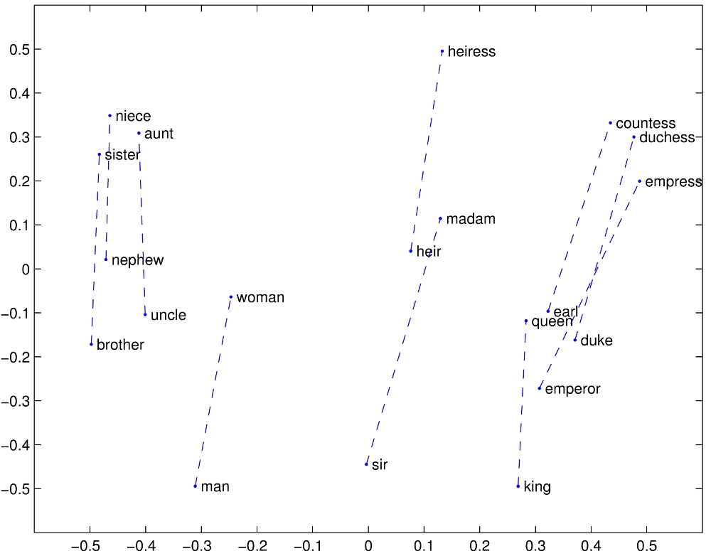
For this part of the assignment, we will try to duplicate their experiments. Given the GloVe vectors and a set of words with some semantic relationship, e.g. (male, female) nouns, we will plot the vector for each word and draw line connecting the two.
Plotting multidimensional GloVe vectors
We’d like to be able take a bunch of GloVe vectors and make a 2D plot. Of course, our GloVe vectors are anywhere from 50 to 300 dimensions long, so we can’t just plot that directly. Instead, we will use two tools: principal component analysis (PCA), and t-distributed Stochastic Neighbor Embedding (t-SNE) to reduce the dimensionality of the vectors down to 2. You don’t need to understand how PCA or t-SNE works, but you might find that skimming through these short introduction to PCA and introduction to t-SNE websites helpful for understanding how things are working.
We’ll start by explaining how to approach this using PCA. We’ll use a similar technique when we switch over to t-SNE.
Extracting the words
We’re going to use scikit-learn
to perform PCA for us. However, we don’t want to perform PCA on all of the
embeddings. Rather, we’re going to extract all the words in the pairs of
related words that we’re interested in and put them into a new,
smaller matrix of embeddings, then we’ll perform PCA on that smaller matrix.
Let’s assume you’ve somehow acquired a list of related words that you’d like to plot. For example:
related = [('brother', 'sister'), ('nephew', 'niece'), ('werewolf', 'werewoman')]You want to go through the array and extract all the rows that match
the words you want to plot. However, you only want to extract the rows
if both words can be found in the array. For example, in the
glove.6B.50d.txt file, the words ‘brother', ‘sister', ‘nephew',
‘niece', and ‘werewolf' appear, but ‘werewoman' doesn’t appear. You’ll
want to extract the vectors only for ‘brother', ‘sister', ‘nephew',
and ‘niece', skipping ‘werewolf' (even though it has a vector) and
‘werewoman' (since it doesn’t have a vector).
Write a function called extract_words that takes two parameters: the
original embeddings (not normalized) and a list of related word pairs.
Your function will create and return a new pandas DataFrame that contains
only the rows for the pairs of words you are extracting.
matrix = extract_words(embeddings, word_pairs)| It will make your life a lot easier if you can extract the words into this new array in the order they appeared in the list of related words. This way, each even-indexed array row is followed by its corresponding pair. In this case, row 0 would be ‘brother', followed by row 1 which would be ‘sister'; row 2 would be ‘nephew', followed by and row 3 which would be ‘niece'. |
Performing PCA
Below is the code needed to perform PCA on your embeddings:
from sklearn.decomposition import PCA  # put this at the top of your program

def perform_pca(matrix):
    # we want to reduce these vectors to 2 dimensions
    model = PCA(n_components=2)
    # learn the transformation and apply it
    reduced = model.fit_transform(matrix)
    # convert it back into a dataframe with columns "x", "y", and matching labels
    df = pd.DataFrame(reduced, columns=["x", "y"], index=matrix.index)
    return df

reduced_matrix = perform_pca(matrix)
Performing t-SNE
Another common technique for compressing embeddings into two dimensions is t-SNE. The code is nearly identical to the code for PCA shown above. You only need to change the following lines:
from sklearn.manifold import TSNE   # put this at the top of your program

def perform_tsne(matrix):
    # we want to reduce these vectors to 2 dimensions
    model = TSNE(n_components=2, perplexity=5, random_state=0)
The description that follows assumes you are using PCA, but eventually you will have a command-line argument that determines if you are calling PCA or t-SNE.
Plotting the vectors
Assuming that the embeddings you perfomed PCA on is called reduced_matrix
(as in the example above), this section will explain how to write a function
that plots the vectors using matplotlib. To use matplotlib, put this
line at the top of your file:
import matplotlib.pyplot as pltYou will eventually write a function called plot_relations that will take your
reduced_matrix and a filename as its only parameters, and it will plot the vectors,
saving them to the specified file. The function will have no return value.
You can put the code we develop below into the plot_relations function
as we go along, but we’ll develop the solution in pieces.
Let’s start by just plotting the (x,y) coordinate of all of the vectors in the array we just performed PCA on since they are all now two-dimensional vectors.
fig = plt.figure(figsize = (8,8))
ax = fig.add_subplot(1,1,1)
plt.scatter(reduced_matrix['x'], reduced_matrix['y'], c='r', s=50)
plt.savefig(filename)
In the example above, there is the optional argument c which sets the color to
r (red). There is a second optional argument s which sets the size of each
point to 50. You can read the documentation for the matplotlib function
scatter
for more information on those and other options.
brother sister
nephew niece
werewolf werewoman
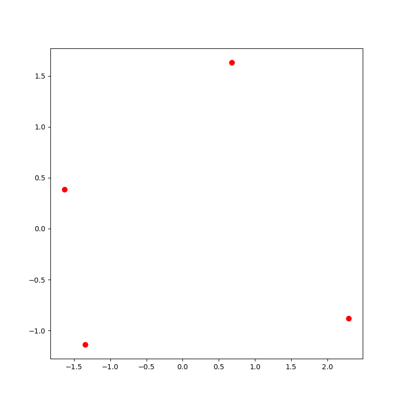
If you started with the list of related words shown above, you should
get the picture below. Notice the picture only has four dots because neither
'werewolf' nor 'werewoman' are in your reduced_matrix.
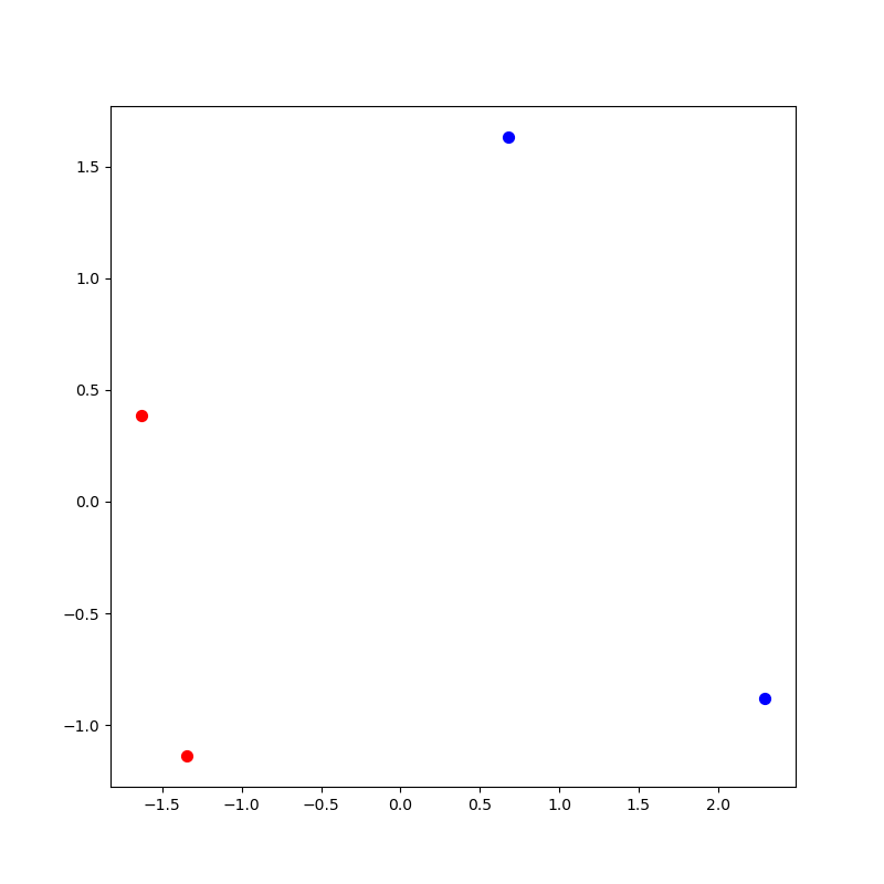
Using alternating colors
We can improve on this picture by making the first half of the each relation
in one color and the second half of each relation in another color.
To do this, make two new lists of integers. In the first list of integers,
store the indexes of the even numbered rows. In the second list of integers,
store the indexes of the odd numbered rows. In this case, the first list
would contain [0, 2] and the second list would contain [1, 3]. In general,
you need to make sure this list scales with the number of rows in your reduced_matrix.
Now try re-plotting as follows, where evens and odds are the two lists
described above:
plt.scatter(reduced_matrix.iloc[evens]['x'], reduced_matrix.iloc[evens]['y'], c='r', s=50)
plt.scatter(reduced_matrix.iloc[odds]['x'], reduced_matrix.iloc[odds]['y'], c='b', s=50)
If you are successful, you should have a picture that looks like this:
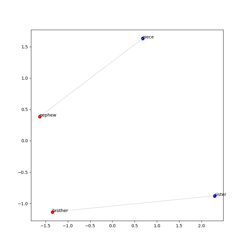
Adding text labels
There are two more important pieces to add in order for us to generate the picture
from the GloVe website. First, let’s add text labels to each of the dots
so we know what each one is representing. The basic idea is we iterate over
each of the row labels (the words) in the reduced_matrix and annotate that (x,y)
coordinate with the label. In the example below, the color of text is set
to k (black).
for i, label in enumerate(reduced_matrix.index):
    plt.annotate(label, (reduced_matrix['x'].iloc[i], reduced_matrix['y'].iloc[i]), color='k')
Connecting pairs of related words
The last piece is to connect pairs of related words with a
line. To do this, we need a line that connects each even-indexed element
in the reduced_matrix with the next odd-indexed element. We’ll do this
using the python function zip:
for even, odd in zip(evens, odds):
    x_values = [reduced_matrix['x'].iloc[even], reduced_matrix['x'].iloc[odd]]
    y_values = [reduced_matrix['y'].iloc[even], reduced_matrix['y'].iloc[odd]]
    plt.plot(x_values, y_values, color='lightgray', linewidth=1)
If your code is working, you should end up with a picture that looks like this:
Completing the visualization
Your visualize.py should have the following command-line interface:
usage: visualize.py [-h] [-o OUTPUT] [--tsne] pickle relations

Plot the relationship between the GloVe vectors for pairs of related words.

positional arguments:
  pickle                path to glove vectors pickle
  relations             a file containing pairs of relations

options:
  -h, --help            show this help message and exit
  -o OUTPUT, --output OUTPUT
                        path to save the plot (default is plot.png)
  --tsne                perform t-SNE (default is PCA)
Your program should read the vectors in the pickle file, read the relations,
then produce a plot like the one shown above. The plot should be saved
in the plot.png unless an --output filename is provided. Your vectors
should be reduced using PCA unless --tsne is given, in which case you
should reduce your vectors using t-SNE.
Questions
-
Plot each of the relations found in the
/data/cs91r-s25/glove/relations/directory. What did you find? Did the plots look like you expected them to look? Were there any anomalous data points? Which ones? Can you explain why? -
Use t-SNE instead of PCA to build the same plots. Are the results better or worse? Discuss.
-
OPTIONAL: t-SNE has a number of parameters you can experiment with. Try changing some of the options to see how it impacts performance. Let us know what you tried and how it turned out!
-
Make your own relations files with ideas that you have about words you think might follow a similar pattern to the ones you’ve seen. You decide how many words are in the file and what the words are. Save the images of the plots you make and include them in your writeup. Try using both PCA and t-SNE.
-
Answer the same kinds of questions you did before, e.g. What did you find? Is it what you expected? etc.
-
Repeat for as many as you’d like, but at least 2 different sets of relations files would help you see if there are patterns.
-
-
Choose one (or more) of the relations we provided for you and replot them using PCA and t-SNE using the other embedding files. Report on what you learn!
-
glove.42B.300d.pkl -
glove.840B.300d.pkl -
GoogleNews-vectors-negative300.pkl
-
Predictive pictures
In the final part of the lab, we will write our code in predict.py.
You might be impressed by some of the plots you made. These plots illustrate that some pairs of words seem to have a consistent relationship between them that you can visualize as a new vector connecting the two data points.
A question you might be asking at this point is: do these connecting vectors have predictive power? That is, if you found the vector that connected 'France' to ‘Paris', could you use that information to figure out what the capital of ‘Hungary' was?
We will need to re-use the extract_words function from visualize.py.
You should either import this from visualize.py or just copy it over.
You will also need to re-use the cosine and normalize functions
from cosine.py, which you can import or copy over.
Average vector difference
Let’s say we have two vectors, a and b, that correspond to two words in our relations file, say, ‘paris’ and ‘france’. Using the embeddings, we can subtract the vectors to find the vector that connects them:

If you have trouble convincing yourself that this picture is correct, what happens if you add the vector \(b\) to the vector \(a-b\)?
Performing vector subtraction in python is straightforward since our data is in a pandas DataFrame. We can just subtract them:
paris = embeddings.loc['paris']
france = embeddings.loc['france']
difference = paris - france
If we compute this difference for all the pairs in a single relations file, we can then find the average vector that connects the second word in a relation back to the first word. You can visualize the average vector as follows:
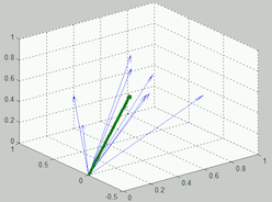
In the picture above, each of the light blue lines is a vector that is the result of computing the vector subtraction show above on one pair of relations. The green line is showing the average of each of those vectors.
Computing an average of vector differences is straightforward. We just put all of the differences in a list, convert them to a DataFrame and calculate the mean:
# assuming vec_lst is a list of vector differences you want to average
df = pd.DataFrame(vec_lst)
average_vector = df.mean(axis=0)
Write a function called average_difference that takes your original embeddings
(without normalizing them or using PCA/t-SNE) and your list of relations,
and returns the average vector
that connects the second word to the first word. Before trying to find the
average, you’ll want to call your extract_words function (from visualize.py)
to be sure you are only including vectors when both pairs in a relation are
present in the GloVe vectors.
Predictive ability
In cosine.py, you wrote code that found the most similar word to words
like ‘red’ and ‘jupiter’. Now we’re going to see if we can use the
average vector above to make predictions about how words are related.
Repeat each of the questions below with each of the relations files provided
in the /data/glove/relations/ directory. Your program should work as follows:
usage: predict.py [-h] pickle relations

Determine if relationships have predictive power

positional arguments:
  pickle      path to glove vectors pickle
  relations   a file containing pairs of relations

options:
  -h, --help  show this help message and exit
After reading in the vectors and the relations, perform the following steps:
-
Given a list of relations,
shufflethe list so that the order that they appear in the list is randomized. Pairs of words should remain together! -
Create a list called
training_relationsthat contains the first 80% of the relations in this shuffled list. (Round, as necessary, if your list isn’t evenly divisible). -
Create a list called
test_relationsthat contains the last 20% of the relations in this shuffled list. Yourtraining_relationsandtest_relationslists should not contain any overlapping pairs and, between them, should contain all of the original relations. -
Using your
average_differencefunction, find the average difference between all of the words in yourtraining_relations. Let’s call this average differenceavg_diff. (We will use this in Question 11 below.)
Note: You are welcome to use the train_test_split function for parts 1-3 above.
Questions
-
Ignore the average vector for this question. Normalize your embeddings using your
normalizefunction. For each vector representing the second word in thetest_relations, use cosine similarity (with yourcosinefunction) to find the most similar vectors/words. Be sure to exclude the result for the word you looked up since this will always be the first result. (NOTE: What happens if the first word and second word are the same? Be careful!)-
How often is the first word in the relation the most similar word to the second word?
-
How often is the first word in the relation in the top 10 most similar words?
-
Report the average position you found the first word in the results.
-
-
For each vector representing the second word in the
test_relations, add theavg_diffvector computed above to this vector. Be sure to use the original un-normalized embeddings when adding these vectors together. This will make a new vector whose length you do not know, so be sure to normalize it usingnumpy.linalg.norm. Once you have this new normalized vector, use yourcosinefunction to compare it to the normalized embeddings.-
How often is the first word in the relation the most similar word to the second word?
-
How often is the first word in the relation in the top 10 most similar words?
-
Report the average position you found the first word in the results.
-
-
What did you just do? Explain in your own words what these two questions accomplished, if anything. Are you surprised at the results? If so, why? If not, why not?
-
Repeat this experiment a couple times because your training and testing sets were randomized and you will get different results each time you run it. Were there large differences between runs?
-
Repeat the above experiments for the relations files that you created to see how this technique works on those pairs of words. Did you get similar results for your pairs of words?
-
Repeat Q10, Q11, and Q12 using the other embedding files. How do your results change? Are there any interesting differences? Share any/all observations you have made.
-
glove.42B.300d.pkl -
glove.840B.300d.pkl -
GoogleNews-vectors-negative300.pkl
-
-
OPTIONAL: Does the algorithm perform the same, better or worse if you flip columns A and B in the relations files?
-
OPTIONAL: Experiment! Are there other ideas/techniques that you want to try? Let us know what you tried and what you found!
How to turn in your solutions
Edit the README.md file that we provided to answer each of the questions
and add any discussion you think we’d like to know about.
Be sure to commit and push all changes to your python files.
If you think it would be helpful, use asciinema to record
a terminal session and include it your README.md.