Your counts.py program should use functions you already created: tokenize, words_by_frequency, and filter_nonwords. Your program should read from a file, if provided as a command-line argument, or read from standard in if no file is provided on the command-line.

Your program should also optionally accept the command-line argument -l, which determines whether or not to lowercase all of the words before counting, and the command-line argument -w, which determines whether or not to keep only the words (filtering the non-words). Both -l and -w can be present, and you can assume that if they are provided on the command-line, they are provided before the filename.

The counts.py program will count the words in the text and print to standard out. The words should be printed from most frequent to least frequent. (Words with the same frequency can be printed in any order.) The output should contain, on each line, a single word, followed by a tab, followed by the count of that word.

Your program should gracefully handle the case where it’s output is piped to head by catching the BrokenPipeError. See the slides from lecture 3 for the specific syntax to do that.

Here are some examples of the program running:

Do not continue to the next section until this is working.

We will be exploring the relationship between the frequency of a token and the rank of that token. You can use your counts.py program to count the lowercased words in carroll-alice.txt to get this result:

Given these results, we would say that the comma , has a rank of 1 since it was the most frequent token, the word the has a rank of 2 since it was the second-most frequent token, the open quotation mark “ has a rank of 3, and so on.

Let \(f\) be the relative frequency of the word and \(r\) be the rank of that word. Assuming you lower-cased the text and didn’t filter out non-words, the word the occurs 1643 times out of 35830 tokens so \(f_{\text{the}} = \frac{1643}{35830} = 0.045855\). Since the was the 2nd most frequent word, \(r_{\text{the}}=2\).

To visualize the relationship between rank and frequency, we will create a log-log plot of rank (on the x-axis) versus frequency (on the y-axis). We will use the pylab library, part of matplotlib:

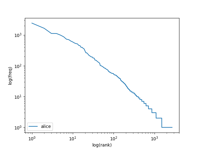
To run your program, use the output of your counts.py program as input to your zipf.py program. As a command-line argument, provide a name for your data. Use the name as a replacement for the variable label in the code above.

Now we can test how well Zipf’s law works.

To do so, we will plot the rank vs. empirical frequency data (as we just did above) and also plot the rank vs. expected frequencies using Zipf’s law. For the constant \(k\) in the formulation of Zipf’s law above, you should use \(\frac{T}{H(n)}\) where \(T\) is the number of tokens in the corpus, \(n\) is the number of types in the corpus, and \(H(n)\) is the \(n\)th harmonic number, which you can calcuate using this function:

According to Zipf’s law, and using our calculated value for \(k\), we get the following: \(f = \frac{k}{r} = \frac{\frac{T}{H(n)}}{r} = \frac{T}{H(n)*r}\)

With this formula, for any rank, \(r\), you can now predict the expected frequency, \(f\), as predicted by Zipf’s law.

To plot a second curve, simply add a second pylab.loglog(…​) line immediately after the line shown in the example above.

We’ll use the counts from "the Gutenberg corpus" that we created Question 4 above. We won’t use the Google ngram corpus in this question because it contains too many misspellings and nonsense words.

To start, we need to calculate the probability of seeing a word in a corpus. To do so, we simply count how many times the word occurred in the corpus and divide it by the total number word tokens in the text. (Be sure to use word tokens and not word types.) In the equation below, \(w\) is a variable used to represent a single word in the text:

Calculate the probability \(p_\text{hamlet}(w)\) for every word in the Hamlet corpus, and calculate \(p_\text{google}(w)\) for every word in the Google corpus in the same way:

Note: The probabilities you will calculate are very small. For example, the probability of seeing the word apple, a fairly common English word, is just 0.000012 in the Google corpus. For less common words like yellowness, the probabilty is 0.000000092.

A common way to compare two probabilities is to calculate a Log Odds Ratio. To calculate the Log Odds Ratio, we calculate the probability of seeing a word in the Hamlet text and divide it by the probability of the same word in the Google corpus, then take the \(log\) of that ratio.

It doesn’t make sense for us to just subtract the two probabilities and calculate the difference because the probabilities are so small.

Instead, we will find the ratio of one probability to the other and then take the \(log\). For ratios that are greater than 1, the \(log\) will return a positive number. For ratios that are less than 1, the \(log\) will return a negative number.

Assuming you’ve calculated the probabilities for every word in both corpuses as described in the previous section, you can calculate the Log Odds Ratio as follows:

Notice that it is a problem if \(p_\text{google}(w) = 0\), since you’d be dividing by zero. It’s also a problem if \(p_\text{hamlet}(w)=0\) since you would then need to compute \(\log(0)\), which is undefined.

To make sure neither of these happen, we will add a very small number, \(\epsilon\), to the top and bottom of the ratio. When we do this, we say we are smoothing the data. In particular, this particular method of smoothing is called LaPlace smoothing or additive smoothing.

Let’s set \(\epsilon = 0.00001\) and recalculate the Smoothed Log Odds Ratio:

To run your logodds.py program, you will provide two files as command-line arguments. Each file will contain the counts in the same format as you made using counts.py. For example, to compare Hamlet to Alice in Wonderland, you could say this:

Rather than reading your counts into a list of tuples, you will need to read your counts into a python dictionary, that way you can easily look up the count for any word in both corpora.

Compare "Alice in Wonderland" to "Hamlet".

Now we’ll compare all three of Shakespeare’s plays (in that directory) to the entire Google ngrams counts. That should give us a sense of the kind of words that Shakespeare used that are different than other book authors. To do that without uncompressing your ngrams counts file, you’ll need to do something like this (assuming your Shakespeare counts are in shakespeare.txt and your compressed google counts are in /scratch/user1/all_sorted.txt.gz)

This may a minute or so depending on your implementation. There are a lot of words in the ngrams corpus. This will also generate a lot of output, so you should save the output to a file in your /scratch directory. Do not check this output file into your repository!